Matplotlib | Show formulas in TeX font (mathtext)

Are you wondering how to display a formula on a graph? You need to show formulas to improve the interpretation of your data and the readability of your graphs.

This article details how to use Matplotlib’s mathtext feature to show formulas on a graph. This allows mathematical relationships and patterns to be shown directly on the graph.

It also explains how to use formulas in TeX fonts.

You can gain clearer communication and insight by visually presenting mathematical concepts and functions in your projects and reports.

Show strings on the plot area (Axes.text)

Axes.text shows the formula on the plot area

Below are the parameters, return values, and links to the official documentation

Show formulas on the plot area

The formulas are 4 + 2sin(2x) and 4 + 2cos(2x)

Each formula is replaced by the variables tex1 and tex2 as row strings enclosed in $.

The following tabs explain the code and flowchart

import matplotlib.pyplot as plt
import numpy as np

# step1 Create data
x = np.linspace(0, 10, 100)
y1 = 4 + 2 * np.sin(2 * x)
y2 = 4 + 2 * np.cos(2 * x)
# step2 Create graph frames
fig, ax = plt.subplots()
# step3 Plot a graph with Axes.plot
ax.plot(x, y1, linestyle=self.line_styles[0], label='Sample 1')
ax.plot(x, y2, linestyle=self.line_styles[1], label='Sample 2')
# step4 Show texts with Axes.text
tex1 = r'$4+2{\rm sin}(2x)$'
tex2 = r'$4+2{\rm cos}(2x)$'
ax.text(0.2, 1, tex1, fontsize=20, va='bottom', color='C0')
ax.text(0.2, 0.2, tex2, fontsize=20, va='bottom', color='C1')
        
ax.set_xlim(0, 8)
ax.set_ylim(0, 8)
ax.set_xlabel('Time [sec]')
ax.set_ylabel('Frequency [Hz]')
ax.legend()

plt.show()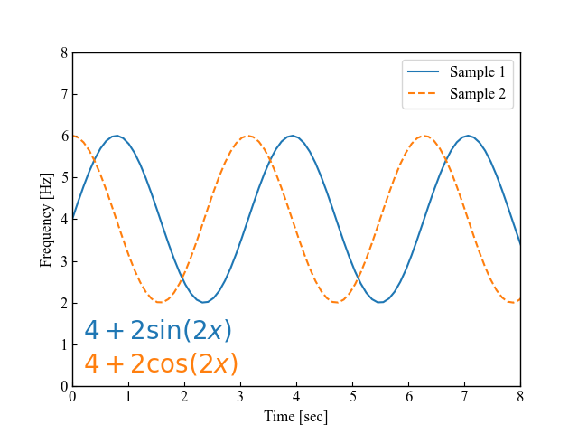

Show formulas in graph titles and axis labels

It also displays formulas in the graph title (ax.set_title) and axis labels (ax.set_xlabel, ax.set_ylabel)

Any row string enclosed in $ will be considered a formula

# step4 Show texts with Axes.text
tex1 = r'$4+2{\rm sin}(2x)$'
tex2 = r'$4+2{\rm cos}(2x)$'

ax.text(0.2, 1, tex1, fontsize=20, va='bottom', color='C0')
ax.text(0.2, 0.2, tex2, fontsize=20, va='bottom', color='C1')

# Axis label
ax.set_xlabel('Time [sec]'r'$\Delta_i^j$')
ax.set_ylabel('Frequency [Hz]'r'$\Delta_i^j$')
# Title
ax.set_title(r"$W^{3\beta}_{\delta_1 \rho_1} = "
r"U^{3\beta}_{\delta_1 \rho_1} + \frac{1}{8 \pi^{2}} $")

plt.show()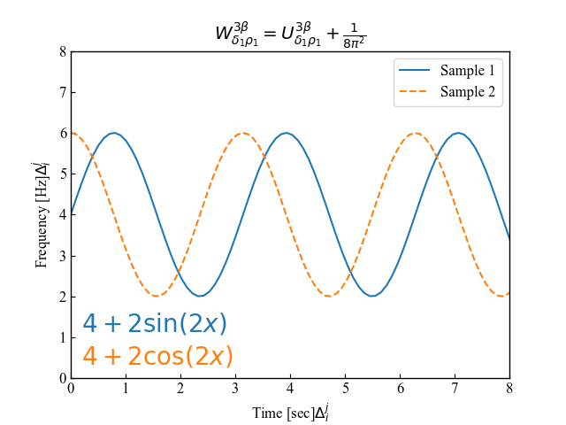

Customize Formula Fonts

Matplotlib formula input is applied by enclosing the row string in $.

Matplotlib does not require TeX to be installed. The layout engine is almost directly based on Donald Knuth’s TeX layout algorithm, so the quality is quite good.

Specifies the formatting of formula text

Normal text and mathtext can be mixed in the same string

The following is a list of typical fonts discussed in this article

The following tabs explain the code and flowchart

# step1 Create data
x = np.linspace(0, 10, 100)
y1 = 4 + 2 * np.sin(2 * x)
y2 = 4 + 2 * np.cos(2 * x)
y3 = 6 + 2 * np.sin(2 * x)
y4 = 6 + 2 * np.cos(x)
# step2 Create graph frames
fig, ax = plt.subplots()
# step3 Plot graphs with Axes.plot
ax.plot(x, y1, linestyle=self.line_styles[0])
ax.plot(x, y2, linestyle=self.line_styles[1])
ax.plot(x, y3, linestyle=self.line_styles[2])
ax.plot(x, y4, linestyle=self.line_styles[3])
# step4 Show texs with Axes.text
tex1 = r'Computer Modern. $Computer Modern. 4+2{\rm sin}(2x)$'
tex2 = r'Dejavu Sans. $Dejavu Sans. 4+2{\rm cos}(2x)$'
tex3 = r'Dejavu Serif. $Dejavu Serif. 6+2{\rm sin}(2x)$'
tex4 = r'Stix Sans. $Stix Sans. 6+2{\rm cos}(x)$'

ax.text(0.2, 0.2, tex1, color='C0', math_fontfamily='cm', size=16)
ax.text(0.2, -1, tex2, color='C1', math_fontfamily='dejavusans', size=16)
ax.text(0.2, -2.2, tex3, color='C2', math_fontfamily='dejavuserif', size=16)
ax.text(0.2, -3.4, tex4, color='C3', math_fontfamily='stixsans', size=16)
    
plt.show()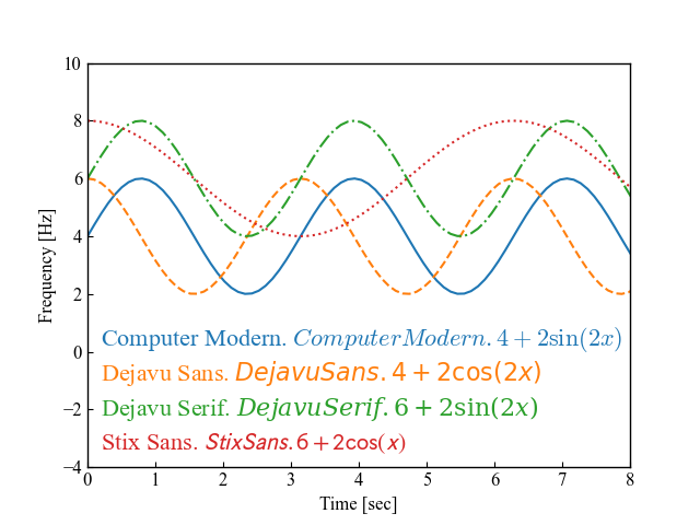

Make TeX fonts default with rcPrams

The mathtext font can be selected with the customization variable mathtext.fontset

Set the mathtext font in plt.rcParams[‘mathtext.fontset’].

import matplotlib.pyplot as plt
import numpy as np

plt.rcParams['mathtext.fontset'] = 'cm'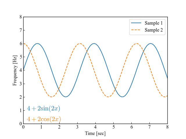

Demonstration of formula display

There are many different types of formulas, but this section explains how to show some of the most commonly used formulas.

subscript and superscript

Use underscores “_” for subscripts and carets “^” for superscripts.

If two or more characters are present, they can be combined into a single block using {}.

fig, ax = plt.subplots()

subscripts_superscripts = [
    'alpha > beta', 
    r'$\alpha > \beta$', 
    r'$\alpha^{ic} > \beta_{ic}$', 
    r'$\sum_{i=0}^\infty x_i$'
]

for i, tex in enumerate(subscripts_superscripts):
    ax.text(0.5, i*1.5+2, tex, size=18)

plt.show()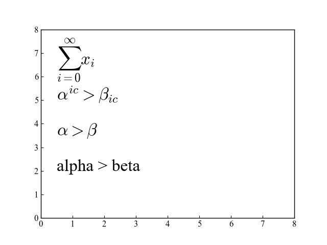

fraction

Fractions are denoted by \frac{numerator}{denominator}

Similar expressions to fractions are binomial and stacked numbers, denoted by\binom{}{} and\genfrac{}{}{}{}, respectively.

The fractional brackets should bracket the entire expression using the brackets \left and \right

fig, ax = plt.subplots()

fractions = [
    r'$\frac{3}{4} \binom{3}{4} \genfrac{}{}{0}{}{3}{4}$',
    r'$\frac{5 - \frac{1}{x}}{4}$',
    r'$(\frac{5 - \frac{1}{x}}{4})$',
    r'$\left(\frac{5 - \frac{1}{x}}{4}\right)$'
]

for i, tex in enumerate(fractions):
    ax.text(0.5, i*1.5+2, tex, size=18)
    
plt.show()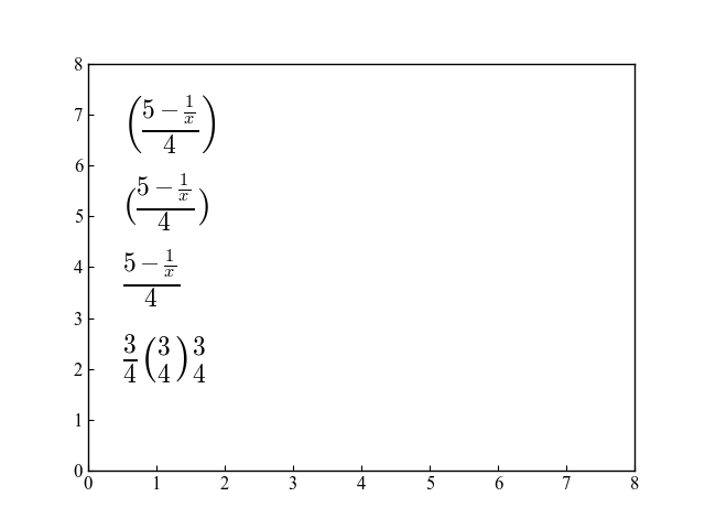

square root

Square roots can be entered using \sqrt

Multipliers for square roots can be entered using [].

fig, ax = plt.subplots()

radicals = [
    r'$\sqrt{2}$',
    r'$\sqrt[3]{x}$'
]

for i, tex in enumerate(radicals):
    ax.text(0.5, i*1.5+2, tex, size=18)
    
plt.show()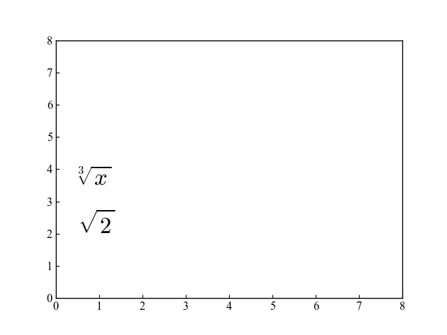

References

Axes.text function

Demonstration of formula text

Summary of formula expressions